CSOUND Español
PHYSICAL MODELLING
MODELADO FISICO
With physical modelling we employ a completely different approach to synthesis than we do with all other standard techniques. Unusually the focus is not primarily to produce a sound, but to model a physical process and if this process exhibits certain features such as periodic oscillation within a frequency range of 20 to 20000 Hz, it will produce sound.
Con el modelado físico empleamos un enfoque de síntesis completamente diferente al que hacemos con todas las otras técnicas estándar. Inusualmente el foco no es principalmente producir un sonido, sino modelar un proceso físico y si este proceso exhibe ciertas características tales como oscilación periódica dentro de un rango de frecuencia de 20 a 20000 Hz, producirá sonido.
Physical modelling synthesis techniques do not build sound using wave tables, oscillators and audio signal generators, instead they attempt to establish a model, as a system in itself, which can then produce sound because of how the system varies with time. A physical model usually derives from the real physical world, but could be any time-varying system. Physical modelling is an exciting area for the production of new sounds.
Las técnicas de síntesis de modelado físico no construyen el sonido usando tablas de onda, osciladores y generadores de señales de audio, sino que intentan establecer un modelo, como un sistema en sí mismo, que puede producir sonido debido a cómo el sistema varía con el tiempo. Un modelo físico normalmente deriva del mundo físico real, pero podría ser cualquier sistema variable en el tiempo. El modelado físico es un área emocionante para la producción de nuevos sonidos.
Compared with the complexity of a real-world physically dynamic system a physical model will most likely represent a brutal simplification. Nevertheless, using this technique will demand a lot of formulae, because physical models are described in terms of mathematics. Although designing a model may require some considerable work, once established the results commonly exhibit a lively tone with time-varying partials and a "natural" difference between attack and release by their very design - features that other synthesis techniques will demand more from the end user in order to establish.
Comparado con la complejidad de un sistema físicamente dinámico del mundo real, un modelo físico probablemente representará una simplificación brutal. Sin embargo, el uso de esta técnica exigirá muchas fórmulas, porque los modelos físicos se describen en términos de matemáticas. Aunque el diseño de un modelo puede requerir un trabajo considerable, una vez establecidos los resultados comúnmente muestran un tono vivo con particiones variables en el tiempo y una diferencia natural entre ataque y liberación por su propio diseño - características que otras técnicas de síntesis requerirán más del usuario final en Para establecer.
Csound already contains many ready-made physical models as opcodes but you can still build your own from scratch. This chapter will look at how to implement two classical models from first principles and then introduce a number of Csound's ready made physical modelling opcodes.
Csound ya contiene muchos modelos físicos ya preparados como opcodes, pero todavía puede construir su propio desde cero. En este capítulo veremos cómo implementar dos modelos clásicos a partir de los primeros principios y luego introducir un número de opcodes de modelado físico preparados de Csounds.
The Mass-Spring Model1
El modelo masa-Resorte1
Many oscillating processes in nature can be modelled as connections of masses and springs. Imagine one mass-spring unit which has been set into motion. This system can be described as a sequence of states, where every new state results from the two preceding ones. Assumed the first state a0 is 0 and the second state a1 is 0.5. Without the restricting force of the spring, the mass would continue moving unimpeded following a constant velocity:
Muchos procesos oscilantes en la naturaleza pueden modelarse como conexiones de masas y resortes. Imagínese una unidad de masa-resorte que ha sido puesta en movimiento. Este sistema puede ser descrito como una secuencia de estados, donde cada nuevo estado resulta de los dos precedentes. Suponiendo que el primer estado a0 es 0 y el segundo estado a1 es 0,5. Sin la fuerza restrictiva del resorte, la masa seguiría moviéndose sin obstáculos siguiendo una velocidad constante:
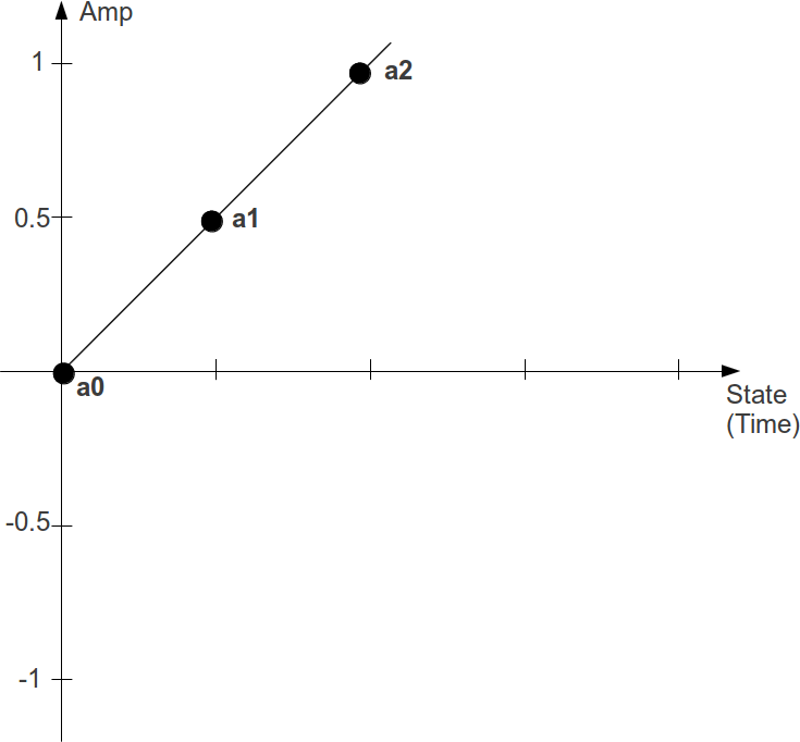
As the velocity between the first two states can be described as a1-a0, the value of the third state a2 will be:
Como la velocidad entre los dos primeros estados se puede describir como a1-a0, el valor del tercer estado a2 será:
a2 = a1 + (a1 - a0) = 0.5 + 0.5 = 1
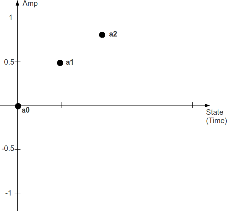
But, the spring pulls the mass back with a force which increases the further the mass moves away from the point of equilibrium. Therefore the masses movement can be described as the product of a constant factor c and the last position a1. This damps the continuous movement of the mass so that for a factor of c=0.4 the next position will be:
Pero el muelle retira la masa con una fuerza que aumenta cuanto más lejos se aleja la masa del punto de equilibrio. Por lo tanto, el movimiento de masas se puede describir como el producto de un factor constante cy la última posición a1. Esto amortigua el movimiento continuo de la masa de modo que para un factor de c = 0,4 la siguiente posición será:
a2 = (a1 + (a1 - a0)) - c * a1 = 1 - 0.2 = 0.8
Csound can easily calculate the values by simply applying the formulae. For the first k-cycle2 , they are set via the init opcode. After calculating the new state, a1 becomes a0 and a2 becomes a1 for the next k-cycle. In the next csd the new values will be printed five times per second (the states are named here as k0/k1/k2 instead of a0/a1/a2, because k-rate values are needed for printing instead of audio samples).
Csound puede calcular fácilmente los valores simplemente aplicando las fórmulas. Para el primer ciclo k2, se establecen a través del código de operación init. Después de calcular el nuevo estado, a1 se convierte en a0 y a2 se convierte en a1 para el siguiente ciclo k. En el siguiente csd los nuevos valores se imprimirán cinco veces por segundo (los estados se nombran aquí como k0 / k1 / k2 en lugar de a0 / a1 / a2, porque los valores de k-rate son necesarios para imprimir en lugar de muestras de audio).
EXAMPLE 04G01_Mass_spring_sine.csd
<CsoundSynthesizer>
<CsOptions>
-n ;no sound
</CsOptions>
<CsInstruments>
sr = 44100
ksmps = 8820 ;5 steps per second

instr PrintVals
;initial values
kstep init 0
k0 init 0
k1 init 0.5
kc init 0.4
;calculation of the next value
k2 = k1 + (k1 - k0) - kc * k1
printks "Sample=%d: k0 = %.3f, k1 = %.3f, k2 = %.3f\n", 0, kstep, k0, k1, k2
;actualize values for the next step
kstep = kstep+1
k0 = k1
k1 = k2
endin

</CsInstruments>
<CsScore>
i "PrintVals" 0 10
</CsScore>
</CsoundSynthesizer>
;example by joachim heintz
The output starts with:
State=0:  k0 =  0.000,  k1 =  0.500,  k2 =  0.800
State=1:  k0 =  0.500,  k1 =  0.800,  k2 =  0.780
State=2:  k0 =  0.800,  k1 =  0.780,  k2 =  0.448
State=3:  k0 =  0.780,  k1 =  0.448,  k2 = -0.063
State=4:  k0 =  0.448,  k1 = -0.063,  k2 = -0.549
State=5:  k0 = -0.063,  k1 = -0.549,  k2 = -0.815
State=6:  k0 = -0.549,  k1 = -0.815,  k2 = -0.756
State=7:  k0 = -0.815,  k1 = -0.756,  k2 = -0.393
State=8:  k0 = -0.756,  k1 = -0.393,  k2 =  0.126
State=9:  k0 = -0.393,  k1 =  0.126,  k2 =  0.595
State=10: k0 =  0.126,  k1 =  0.595,  k2 =  0.826
State=11: k0 =  0.595,  k1 =  0.826,  k2 =  0.727
State=12: k0 =  0.826,  k1 =  0.727,  k2 =  0.337

So, a sine wave has been created, without the use of any of Csound's oscillators... Here is the audible proof:
Así, se ha creado una onda sinusoidal sin el uso de ninguno de los osciladores Csounds ... Aquí está la prueba audible:
EXAMPLE 04G02_MS_sine_audible.csd
<CsoundSynthesizer>
<CsOptions>
-odac
</CsOptions>
<CsInstruments>
sr = 44100
ksmps = 1
nchnls = 2
0dbfs = 1

instr MassSpring
;initial values
a0        init      0
a1        init      0.05
ic        =         0.01 ;spring constant
;calculation of the next value
a2        =         a1+(a1-a0) - ic*a1
          outs      a0, a0
;actualize values for the next step
a0        =         a1
a1        =         a2
endin
</CsInstruments>
<CsScore>
i "MassSpring" 0 10
</CsScore>
</CsoundSynthesizer>
;example by joachim heintz, after martin neukom
As the next sample is calculated in the next control cycle, ksmps has to be set to 1.3 The resulting frequency depends on the spring constant: the higher the constant, the higher the frequency. The resulting amplitude depends on both, the starting value and the spring constant.
Como la siguiente muestra se calcula en el siguiente ciclo de control, ksmps tiene que ser ajustado a 1.3 La frecuencia resultante depende de la constante de resorte: cuanto mayor sea la constante, mayor será la frecuencia. La amplitud resultante depende tanto del valor de arranque como de la constante de muelle.
This simple model shows the basic principle of a physical modelling synthesis: creating a system which produces sound because it varies in time. Certainly it is not the goal of physical modelling synthesis to reinvent the wheel of a sine wave. But modulating the parameters of a model may lead to interesting results. The next example varies the spring constant, which is now no longer a constant:
Este modelo simple muestra el principio básico de una síntesis de modelado físico: crear un sistema que produce sonido porque varía en el tiempo. Ciertamente no es el objetivo de la síntesis de modelado físico reinventar la rueda de una onda sinusoidal. Pero la modulación de los parámetros de un modelo puede dar lugar a resultados interesantes. El siguiente ejemplo varía la constante de muelle, que ya no es una constante:
EXAMPLE 04G03_MS_variable_constant.csd
<CsoundSynthesizer>
<CsOptions>
-odac
</CsOptions>
<CsInstruments>
sr = 44100
ksmps = 1
nchnls = 2
0dbfs = 1

instr MassSpring
;initial values
a0        init      0
a1        init      0.05
kc        randomi   .001, .05, 8, 3
;calculation of the next value
a2        =         a1+(a1-a0) - kc*a1
          outs      a0, a0
;actualize values for the next step
a0        =         a1
a1        =         a2
endin
</CsInstruments>
<CsScore>
i "MassSpring" 0 10
</CsScore>
</CsoundSynthesizer>
;example by joachim heintz
Working with physical modelling demands thought in more physical or mathematical terms: examples of this might be if you were to change the formula when a certain value of c had been reached, or combine more than one spring.
Trabajar con modelos físicos requiere pensamiento en términos más físicos o matemáticos: ejemplos de esto podrían ser si cambiaran la fórmula cuando se alcanzara un cierto valor de c, o combinaran más de una primavera.
Implementing Simple Physical Systems
Implementación de sistemas físicos simples
This text shows how to get oscillators and filters from simple physical models by recording the position of a point (mass) of a physical system. The behavior of a particle (mass on a spring, mass of a pendulum, etc.) is described by its position, velocity and acceleration. The mathematical equations, which describe the movement of such a point, are differential equations. In what follows, we describe how to derive time discrete system equations (also called difference equations) from physical models (described by differential equations). At every time step we first calculate the acceleration of a mass and then its new velocity and position. This procedure is called Euler's method and yields good results for low frequencies compared to the sampling rate (better approximations are achieved with the improved Euler's method or the Runge–Kutta methods).
Este texto muestra cómo obtener osciladores y filtros de modelos físicos simples registrando la posición de un punto (masa) de un sistema físico. El comportamiento de una partícula (masa sobre un resorte, masa de un péndulo, etc.) se describe por su posición, velocidad y aceleración. Las ecuaciones matemáticas, que describen el movimiento de tal punto, son ecuaciones diferenciales. En lo que sigue, describimos cómo derivar ecuaciones discretas de sistemas de tiempo (también llamadas ecuaciones de diferencias) a partir de modelos físicos (descritos por ecuaciones diferenciales). En cada paso de tiempo primero calculamos la aceleración de una masa y luego su nueva velocidad y posición. Este procedimiento se denomina método de Eulers y produce buenos resultados para frecuencias bajas en comparación con la velocidad de muestreo (se obtienen mejores aproximaciones con el método de Eulers mejorado o con los métodos de Runge-Kutta).
The figures below have been realized with Mathematica.
Las siguientes figuras se han realizado con Mathematica.
Integrating the Trajectory of a Point
Integración de la trayectoria de un punto
Velocity v is the difference of positions x per time unit T, acceleration a the difference of velocities v per time unit T:
La velocidad v es la diferencia de posiciones x por unidad de tiempo T, aceleración a la diferencia de velocidades v por unidad de tiempo T:
vt = (xt – xt-1)/T, at = (vt – vt-1)/T.
Putting T = 1 we get
vt = xt – xt-1, at = vt – vt-1.
If we know the position and velocity of a point at time t – 1 and are able to calculate its acceleration at time t we can calculate the velocity vt and the position xt at time t:
Si conocemos la posición y la velocidad de un punto en el tiempo t - 1 y somos capaces de calcular su aceleración en el tiempo t podemos calcular la velocidad vt y la posición xt en el tiempo t:
vt = vt-1 + at andxt = xt-1 + vt
With the following algorithm we calculate a sequence of successive positions x:
Con el siguiente algoritmo calculamos una sucesión de posiciones sucesivas x:
1. init x and v
2. calculate a
3. v += a   	; v = v + a
4. x += v	; x = x + v
Example 1: The acceleration of gravity is constant (g = –9.81ms-2). For a mass with initial position x = 300m (above ground) and velocity v = 70ms-1 (upwards) we get the following trajectory (path)
Ejemplo 1: La aceleración de la gravedad es constante (g = -9,81ms-2). Para una masa con posición inicial x = 300m (sobre el suelo) y velocidad v = 70ms-1 (hacia arriba) se obtiene la siguiente trayectoria (trayectoria)
g = -9.81; x = 300; v = 70; Table[v += g; x += v, {16}];
Example 2: The acceleration a of a mass on a spring is proportional (with factor –c) to its position (deflection) x.
Ejemplo 2: La aceleración a de una masa sobre un resorte es proporcional (con el factor -c) a su posición (deflexión) x.
x = 0; v = 1; c = .3; Table[a = -c*x; v += a; x += v, {22}];
Introducing damping
Introducción al amortiguamiento
Since damping is proportional to the velocity we reduce velocity at every time step by a certain amount d:
Puesto que el amortiguamiento es proporcional a la velocidad, reducimos la velocidad en cada paso del tiempo en una cierta cantidad d:
v *= (1 - d)
Example 3: Spring with damping (see lin_reson.csd below):
Ejemplo 3: Muelle con amortiguación (véase lin_reson.csd a continuación):
d = 0.2; c = .3; x = 0; v = 1;
Table[a = -c*x; v += a; v *= (1 - d); x += v, {22}];
The factor c can be calculated from the frequency f:
El factor c se puede calcular a partir de la frecuencia f:
c = 2 – sqrt(4 – d2) cos(2π f/sr)
Introducing excitation
Introducción de la excitación
In the examples 2 and 3 the systems oscillate because of their initial velocity v = 1. The resultant oscillation is the impulse response of the systems. We can excite the systems continuously by adding a value exc to the velocity at every time step.
En los ejemplos 2 y 3 los sistemas oscilan debido a su velocidad inicial v = 1. La oscilación resultante es la respuesta de impulso de los sistemas. Podemos excitar los sistemas continuamente añadiendo un valor exc a la velocidad en cada paso del tiempo.
v += exc;
Example 4: Damped spring with random excitation (resonator with noise as input)
Ejemplo 4: Muelle amortiguado con excitación aleatoria (resonador con ruido como entrada)
d = .01; s = 0; v = 0; Table[a = -.3*s; v += a; v += RandomReal[{-1, 1}]; v *= (1 - d); s += v, {61}];

EXAMPLE 04G04_lin_reson.csd
<CsoundSynthesizer>
<CsInstruments>
sr = 44100
ksmps = 32
nchnls = 1
0dbfs = 1

opcode 	lin_reson, 	a, akk
setksmps 1
avel 	init 	0 		;velocity
ax 	init 	0 		;deflection x
ain,kf,kdamp 	xin
kc 	= 	2-sqrt(4-kdamp^2)*cos(kf*2*$M_PI/sr)
aacel 	= 	-kc*ax
avel 	= 	avel+aacel+ain
avel 	= 	avel*(1-kdamp)
ax 	= 	ax+avel
	xout 	ax
endop

instr 1
aexc 	rand 	p4
aout 	lin_reson 	aexc,p5,p6
	out 	aout
endin

</CsInstruments>
<CsScore>
; 		p4 		p5 	p6
; 		excitaion 	freq 	damping
i1 0 5 		.0001   	440 	.0001
</CsScore>
</CsoundSynthesizer>
;example by martin neukom
Introducing nonlinear acceleration Example 5: The acceleration of a pendulum depends on its deflection (angle x).
Introducción de aceleración no lineal Ejemplo 5: La aceleración de un péndulo depende de su deflexión (ángulo x).
a = c*sin(x)
This figure shows the function –.3sin(x)
Esta figura muestra la función-3sin (x)
The following trajectory shows that the frequency decreases with encreasing amplitude and that the pendulum can turn around.
La siguiente trayectoria muestra que la frecuencia disminuye con la amplitud creciente y que el péndulo puede girar.
d = .003; s = 0; v = 0;
Table[a = f[s]; v += a; v += RandomReal[{-.09, .1}]; v *= (1 - d);
s += v, {400}];
We can implement systems with accelerations that are arbitrary functions of position x.
Podemos implementar sistemas con aceleraciones que son funciones arbitrarias de la posición x.
Example 6: a = f(x) = – c1x + c2sin(c3x)

d = .03; x = 0; v = 0; Table[a = f[x]; v += a; v += RandomReal[{-.1, .1}]; v *= (1 - d); x += v, {400}];

EXAMPLE 04G05_nonlin_reson.csd
<CsoundSynthesizer>
<CsInstruments>

sr = 44100
ksmps = 32
nchnls = 1
0dbfs = 1

; simple damped nonlinear resonator
opcode nonlin_reson, a, akki
setksmps 1
avel 	init 0			;velocity
adef 	init 0			;deflection
ain,kc,kdamp,ifn xin
aacel 	tablei 	adef, ifn, 1, .5 ;acceleration = -c1*f1(def)
aacel 	= 	-kc*aacel
avel 	= 	avel+aacel+ain	;vel += acel + excitation
avel 	= 	avel*(1-kdamp)
adef 	= 	adef+avel
	xout 	adef
endop

instr 1
kenv 	oscil 		p4,.5,1
aexc 	rand 		kenv
aout 	nonlin_reson 	aexc,p5,p6,p7
	out 		aout
endin

</CsInstruments>
<CsScore>
f1 0 1024 10 1
f2 0 1024 7 -1 510 .15 4 -.15 510 1
f3 0 1024 7 -1 350 .1 100 -.3 100 .2 100 -.1 354 1
; 		p4 		p5 	p6 	p7
;   		excitation  	c1    	damping ifn
i1 0 20   	.0001      	.01   	.00001   3
;i1 0 20  	.0001      	.01   	.00001   2
</CsScore>
</CsoundSynthesizer>
;example by martin neukom
The Van der Pol Oscillator
While attempting to explain the nonlinear dynamics of vacuum tube circuits, the Dutch electrical engineer Balthasar van der Pol derived the differential equation
Al intentar explicar la dinámica no lineal de los circuitos de tubos de vacío, el ingeniero eléctrico holandés Balthasar van der Pol derivó la ecuación diferencial
d2x/dt2 = –ω2x + μ(1 – x2)dx/dt. (where d2x/dt2 = acelleration and dx/dt = velocity)
The equation describes a linear oscillator d2x/dt2 = –ω2x with an additional nonlinear term μ(1 – x2)dx/dt. When |x| > 1, the nonlinear term results in damping, but when |x| < 1, negative damping results, which means that energy is introduced into the system. Such oscillators compensating for energy loss by an inner energy source are called self-sustained oscillators.
La ecuación describe un oscilador lineal d2x / dt2 = -ω2x con un término no lineal adicional μ (1 - x2) dx / dt. Cuando | x | 1, el término no lineal resulta en amortiguamiento, pero cuando | x | 1, los resultados negativos de amortiguación, lo que significa que la energía se introduce en el sistema. Tales osciladores que compensan la pérdida de energía por una fuente de energía interna se denominan osciladores auto sostenidos.
v = 0; x = .001; ω = 0.1; μ = 0.25;
snd = Table[v += (-ω^2*x + μ*(1 - x^2)*v); x += v, {200}];

The constant ω is the angular frequency of the linear oscillator (μ = 0). For a simulation with sampling rate sr we calculate the frequency f in Hz as
La constante ω es la frecuencia angular del oscilador lineal (μ = 0). Para una simulación con tasa de muestreo sr calculamos la frecuencia f en Hz como
f = ω·sr/2π.
Since the simulation is only an approximation of the oscillation this formula gives good results only for low frequencies. The exact frequency of the simulation is
Dado que la simulación es sólo una aproximación de la oscilación esta fórmula da buenos resultados sólo para las frecuencias bajas. La frecuencia exacta de la simulación es
f = arccos(1 – ω2/2)sr·/2π.
We get ω2 from frequency f as
2 – 2cos(f·2π/sr).
With increasing μ the oscillations nonlinearity becomes stronger and more overtones arise (and at the same time the frequency becomes lower). The following figure shows the spectrum of the oscillation for various values of μ.
Con el aumento de μ las oscilaciones la no linealidad se hace más fuerte y más armónicos surgen (y al mismo tiempo la frecuencia se hace más baja). La siguiente figura muestra el espectro de la oscilación para varios valores de μ.

The UDO v_d_p represents a Van der Pol oscillator with a natural frequency kfr and a nonlinearity factor kmu. It can be excited by a sine wave of frequency kfex and amplitude kaex. The range of frequency within which the oscillator is synchronized to the exciting frequency increases as kmu and kaex increase.
El UDO v_d_p representa un oscilador de Van der Pol con una frecuencia natural kfr y un factor de no linealidad kmu. Se puede excitar por una onda senoidal de frecuencia kfex y amplitud kaex. El rango de frecuencia dentro del cual el oscilador está sincronizado con la frecuencia de excitación aumenta a medida que el kmu y el kaex aumentan.
EXAMPLE 04G06_van_der_pol.csd
<CsoundSynthesizer>
<CsOptions>
-odac
</CsOptions>
<CsInstruments>

sr = 44100
ksmps = 32
nchnls = 2
0dbfs = 1

;Van der Pol Oscillator ;outputs a nonliniear oscillation
;inputs: a_excitation, k_frequency in Hz (of the linear part), nonlinearity (0 < mu < ca. 0.7)
opcode v_d_p, a, akk
setksmps 1
av init 0
ax init 0
ain,kfr,kmu xin
kc = 2-2*cos(kfr*2*$M_PI/sr)
aa = -kc*ax + kmu*(1-ax*ax)*av
av = av + aa
ax = ax + av + ain
xout ax
endop

instr 1
kaex = .001
kfex = 830
kamp = .15
kf = 455
kmu linseg 0,p3,.7
a1 poscil kaex,kfex
aout v_d_p a1,kf,kmu
out kamp*aout,a1*100
endin

</CsInstruments>
<CsScore>
i1 0 20
</CsScore>
</CsoundSynthesizer>
;example by martin neukom, adapted by joachim heintz
The variation of the phase difference between excitation and oscillation, as well as the transitions between synchronous, beating and asynchronous behaviors, can be visualized by showing the sum of the excitation and the oscillation signals in a phase diagram. The following figures show to the upper left the waveform of the Van der Pol oscillator, to the lower left that of the excitation (normalized) and to the right the phase diagram of their sum. For these figures, the same values were always used for kfr, kmu and kaex. Comparing the first two figures, one sees that the oscillator adopts the exciting frequency kfex within a large frequency range. When the frequency is low (figure a), the phases of the two waves are nearly the same. Hence there is a large deflection along the x-axis in the phase diagram showing the sum of the waveforms. When the frequency is high, the phases are nearly inverted (figure b) and the phase diagram shows only a small deflection. The figure c shows the transition to asynchronous behavior. If the proportion between the natural frequency of the oscillator kfr and the excitation frequency kfex is approximately simple (kfex/kfr ≅ m/n), then within a certain range the frequency of the Van der Pol oscillator is synchronized so that kfex/kfr = m/n. Here one speaks of higher order synchronization (figure d).
La variación de la diferencia de fase entre la excitación y la oscilación, así como las transiciones entre los comportamientos síncronos, de compresión y asíncronos, se pueden visualizar mostrando la suma de las señales de excitación y oscilación en un diagrama de fases. Las figuras siguientes muestran a la izquierda la forma de onda del oscilador de Van der Pol, a la inferior izquierda la de la excitación (normalizada) ya la derecha el diagrama de fase de su suma. Para estas cifras, siempre se utilizaron los mismos valores para kfr, kmu y kaex. Comparando las dos primeras figuras, se ve que el oscilador adopta la frecuencia de excitación kfex dentro de una gran gama de frecuencias. Cuando la frecuencia es baja (figura a), las fases de las dos ondas son casi las mismas. Por lo tanto, existe una gran deflexión a lo largo del eje x en el diagrama de fases que muestra la suma de las formas de onda. Cuando la frecuencia es alta, las fases están casi invertidas (figura b) y el diagrama de fases muestra sólo una pequeña deflexión. La figura c muestra la transición al comportamiento asíncrono. Si la proporción entre la frecuencia natural del oscilador kfr y la frecuencia de excitación kfex es aproximadamente simple (kfex / kfr ≅ m / n), entonces en un cierto rango la frecuencia del oscilador de Van der Pol se sincroniza de modo que kfex / kfr = Minnesota. Aquí se habla de sincronización de orden superior (figura d).


The Karplus-Strong Algorithm: Plucked String
El Algoritmo Karplus-Fuerte: Cuerda Plegada
The Karplus-Strong algorithm provides another simple yet interesting example of how physical modelling can be used to synthesized sound. A buffer is filled with random values of either +1 or -1. At the end of the buffer, the mean of the first and the second value to come out of the buffer is calculated. This value is then put back at the beginning of the buffer, and all the values in the buffer are shifted by one position.
El algoritmo Karplus-Strong proporciona otro ejemplo sencillo pero interesante de cómo el modelado físico puede ser utilizado para sintetizar el sonido. Un buffer se llena con valores aleatorios de 1 o -1. Al final del buffer, se calcula la media del primer y el segundo valor que sale del búfer. Este valor se vuelve a colocar al principio del búfer y todos los valores del búfer se desplazan en una posición.
This is what happens for a buffer of five values, for the first five steps:
Esto es lo que sucede para un búfer de cinco valores, para los primeros cinco pasos:
| initial state | 1 | -1 | 1 | 1 | -1 |
| step 1 | 0 | 1 | -1 | 1 | 1 |
| step 2 | 1 | 0 | 1 | -1 | 1 |
| step 3 | 0 | 1 | 0 | 1 | -1 |
| step 4 | 0 | 0 | 1 | 0 | 1 |
| step 5 | 0.5 | 0 | 0 | 1 | 0 |
The next Csound example represents the content of the buffer in a function table, implements and executes the algorithm, and prints the result after each five steps which here is referred to as one cycle:
El siguiente ejemplo de Csound representa el contenido del búfer en una tabla de funciones, implementa y ejecuta el algoritmo e imprime el resultado después de cada cinco pasos que aquí se conoce como un ciclo:
EXAMPLE 04G07_KarplusStrong.csd
<CsoundSynthesizer>
<CsOptions>
-n
</CsOptions>
<CsInstruments>
sr = 44100
ksmps = 32
nchnls = 1
0dbfs = 1

  opcode KS, 0, ii
  ;performs the karplus-strong algorithm
iTab, iTbSiz xin
;calculate the mean of the last two values
iUlt      tab_i     iTbSiz-1, iTab
iPenUlt   tab_i     iTbSiz-2, iTab
iNewVal   =         (iUlt + iPenUlt) / 2
;shift values one position to the right
indx      =         iTbSiz-2
loop:
iVal      tab_i     indx, iTab
          tabw_i    iVal, indx+1, iTab
          loop_ge   indx, 1, 0, loop
;fill the new value at the beginning of the table
          tabw_i    iNewVal, 0, iTab
  endop

  opcode PrintTab, 0, iiS
  ;prints table content, with a starting string
iTab, iTbSiz, Sin xin
indx      =         0
Sout      strcpy    Sin
loop:
iVal      tab_i     indx, iTab
Snew      sprintf   "%8.3f", iVal
Sout      strcat    Sout, Snew
          loop_lt   indx, 1, iTbSiz, loop
          puts      Sout, 1
  endop

instr ShowBuffer
;fill the function table
iTab      ftgen     0, 0, -5, -2, 1, -1, 1, 1, -1
iTbLen    tableng   iTab
;loop cycles (five states)
iCycle    =         0
cycle:
Scycle    sprintf   "Cycle %d:", iCycle
          PrintTab  iTab, iTbLen, Scycle
;loop states
iState    =         0
state:
          KS        iTab, iTbLen
          loop_lt   iState, 1, iTbLen, state
          loop_lt   iCycle, 1, 10, cycle
endin

</CsInstruments>
<CsScore>
i "ShowBuffer" 0 1
</CsScore>
</CsoundSynthesizer>
;example by joachim heintz
This is the output:
Cycle 0:   1.000  -1.000   1.000   1.000  -1.000
Cycle 1:   0.500   0.000   0.000   1.000   0.000
Cycle 2:   0.500   0.250   0.000   0.500   0.500
Cycle 3:   0.500   0.375   0.125   0.250   0.500
Cycle 4:   0.438   0.438   0.250   0.188   0.375
Cycle 5:   0.359   0.438   0.344   0.219   0.281
Cycle 6:   0.305   0.398   0.391   0.281   0.250
Cycle 7:   0.285   0.352   0.395   0.336   0.266
Cycle 8:   0.293   0.318   0.373   0.365   0.301
Cycle 9:   0.313   0.306   0.346   0.369   0.333
It can be seen clearly that the values get smoothed more and more from cycle to cycle. As the buffer size is very small here, the values tend to come to a constant level; in this case 0.333. But for larger buffer sizes, after some cycles the buffer content has the effect of a period which is repeated with a slight loss of amplitude. This is how it sounds, if the buffer size is 1/100 second (or 441 samples at sr=44100):
Se puede ver claramente que los valores se suavizan cada vez más de ciclo a ciclo. Como el tamaño del búfer es muy pequeño aquí, los valores tienden a llegar a un nivel constante; En este caso 0.333. Pero para tamaños de tampón más grandes, después de algunos ciclos, el contenido del tampón tiene el efecto de un período que se repite con una ligera pérdida de amplitud. Esto es lo que suena, si el tamaño del búfer es 1/100 segundo (o 441 muestras en sr = 44100):
EXAMPLE 04G08_Plucked.csd
<CsoundSynthesizer>
<CsOptions>
-odac
</CsOptions>
<CsInstruments>
sr = 44100
ksmps =  1
nchnls = 2
0dbfs = 1

instr 1
;delay time
iDelTm    =         0.01
;fill the delay line with either -1 or 1 randomly
kDur      timeinsts
 if kDur < iDelTm then
aFill     rand      1, 2, 1, 1 ;values 0-2
aFill     =         floor(aFill)*2 - 1 ;just -1 or +1
          else
aFill     =         0
 endif
;delay and feedback
aUlt      init      0 ;last sample in the delay line
aUlt1     init      0 ;delayed by one sample
aMean     =         (aUlt+aUlt1)/2 ;mean of these two
aUlt      delay     aFill+aMean, iDelTm
aUlt1     delay1    aUlt
          outs      aUlt, aUlt
endin

</CsInstruments>
<CsScore>
i 1 0 60
</CsScore>
</CsoundSynthesizer>
;example by joachim heintz, after martin neukom
This sound resembles a plucked string: at the beginning the sound is noisy but after a short period of time it exhibits periodicity. As can be heard, unless a natural string, the steady state is virtually endless, so for practical use it needs some fade-out. The frequency the listener perceives is related to the length of the delay line. If the delay line is 1/100 of a second, the perceived frequency is 100 Hz. Compared with a sine wave of similar frequency, the inherent periodicity can be seen, and also the rich overtone structure:
Este sonido se asemeja a una cuerda desplumada: al principio el sonido es ruidoso pero después de un corto período de tiempo exhibe periodicidad. Como se puede oír, a menos que una cuerda natural, el estado estacionario es virtualmente sin fin, así que para el uso práctico necesita un cierto fade-hacia fuera. La frecuencia que el oyente percibe está relacionada con la longitud de la línea de retardo. Si la línea de retardo es 1/100 de segundo, la frecuencia percibida es de 100 Hz. En comparación con una onda sinusoidal de frecuencia similar, se puede observar la periodicidad inherente, y también la estructura rica en armónicos:

Csound also contains over forty opcodes which provide a wide variety of ready-made physical models and emulations. A small number of them will be introduced here to give a brief overview of the sort of things available.
Csound también contiene más de cuarenta opcodes que proporcionan una gran variedad de modelos y emulaciones físicas ya hechas. Un pequeño número de ellos se presentará aquí para dar una breve visión general del tipo de cosas disponibles.
wgbow - A Waveguide Emulation of a Bowed String by Perry Cook
Wgbow - Una emulación de guía de ondas de una cuerda arqueada por Perry Cook
Perry Cook is a prolific author of physical models and a lot of his work has been converted into Csound opcodes. A number of these models wgbow, wgflute, wgclar wgbowedbar and wgbrass are based on waveguides. A waveguide, in its broadest sense, is some sort of mechanism that limits the extend of oscillations, such as a vibrating string fixed at both ends or a pipe. In these sorts of physical model a delay is used to emulate these limits. One of these, wgbow, implements an emulation of a bowed string. Perhaps the most interesting aspect of many physical models in not specifically whether they emulate the target instrument played in a conventional way accurately but the facilities they provide for extending the physical limits of the instrument and how it is played - there are already vast sample libraries and software samplers for emulating conventional instruments played conventionally. wgbow offers several interesting options for experimentation including the ability to modulate the bow pressure and the bowing position at k-rate.
Perry Cook es un autor prolífico de modelos físicos y una gran parte de su trabajo se ha convertido en opcodes Csound. Un número de estos modelos wgbow, wgflute, wgclar wgbowedbar y wgbrass se basan en guías de onda. Una guía de ondas, en su sentido más amplio, es una especie de mecanismo que limita la extensión de las oscilaciones, como una cuerda vibradora fija en ambos extremos o una tubería. En estos tipos de modelo físico se usa un retardo para emular estos límites. Uno de estos, wgbow, implementa una emulación de una cuerda inclinada. Quizás el aspecto más interesante de muchos modelos físicos en no específicamente si emulan el instrumento del objetivo jugó de una manera convencional con exactitud pero las facilidades que proporcionan para ampliar los límites físicos del instrumento y cómo lo juega - hay bibliotecas ya extensas de la muestra y Samplers de software para emular instrumentos convencionales jugados convencionalmente. Wgbow ofrece varias opciones interesantes para la experimentación incluyendo la capacidad de modular la presión del arco y la posición de inclinación a la velocidad k.
Varying bow pressure will change the tone of the sound produced by changing the harmonic emphasis. As bow pressure reduces, the fundamental of the tone becomes weaker and overtones become more prominent. If the bow pressure is reduced further the abilty of the system to produce a resonance at all collapse. This boundary between tone production and the inability to produce a tone can provide some interesting new sound effect. The following example explores this sound area by modulating the bow pressure parameter around this threshold. Some additional features to enhance the example are that 7 different notes are played simultaneously, the bow pressure modulations in the right channel are delayed by a varying amount with respect top the left channel in order to create a stereo effect and a reverb has been added.
La variación de la presión del arco cambiará el tono del sonido producido cambiando el énfasis armónico. A medida que la presión del arco se reduce, el fundamental del tono se vuelve más débil y los tonos se vuelven más prominentes. Si la presión del arco se reduce aún más la habilidad del sistema para producir una resonancia en todo colapso. Esta frontera entre la producción de tono y la incapacidad para producir un tono puede proporcionar algún nuevo efecto de sonido interesante. El siguiente ejemplo explora esta área de sonido modulando el parámetro de presión de proa alrededor de este umbral. Algunas características adicionales para mejorar el ejemplo son que se juegan 7 notas diferentes simultáneamente, las modulaciones de presión de arco en el canal derecho se retrasan en una cantidad variable con respecto al canal izquierdo para crear un efecto estéreo y se ha añadido una reverberación.
EXAMPLE 04G09_wgbow.csd
<CsoundSynthesizer>

<CsOptions>
-odac
</CsOptions>

<CsInstruments>

sr      =       44100
ksmps   =       32
nchnls  =       2
0dbfs   =       1
        seed    0

gisine  ftgen	0,0,4096,10,1

gaSendL,gaSendR init 0

 instr 1 ; wgbow instrument
kamp     =        0.3
kfreq    =        p4
ipres1   =        p5
ipres2   =        p6
; kpres (bow pressure) defined using a random spline
kpres    rspline  p5,p6,0.5,2
krat     =        0.127236
kvibf    =        4.5
kvibamp  =        0
iminfreq =        20
; call the wgbow opcode
aSigL	 wgbow    kamp,kfreq,kpres,krat,kvibf,kvibamp,gisine,iminfreq
; modulating delay time
kdel     rspline  0.01,0.1,0.1,0.5
; bow pressure parameter delayed by a varying time in the right channel
kpres    vdel_k   kpres,kdel,0.2,2
aSigR	 wgbow	  kamp,kfreq,kpres,krat,kvibf,kvibamp,gisine,iminfreq
         outs     aSigL,aSigR
; send some audio to the reverb
gaSendL  =        gaSendL + aSigL/3
gaSendR  =        gaSendR + aSigR/3
 endin

 instr 2 ; reverb
aRvbL,aRvbR reverbsc gaSendL,gaSendR,0.9,7000
            outs     aRvbL,aRvbR
            clear    gaSendL,gaSendR
 endin

</CsInstruments>

<CsScore>
; instr. 1
;  p4 = pitch (hz.)
;  p5 = minimum bow pressure
;  p6 = maximum bow pressure
; 7 notes played by the wgbow instrument
i 1  0 480  70 0.03 0.1
i 1  0 480  85 0.03 0.1
i 1  0 480 100 0.03 0.09
i 1  0 480 135 0.03 0.09
i 1  0 480 170 0.02 0.09
i 1  0 480 202 0.04 0.1
i 1  0 480 233 0.05 0.11
; reverb instrument
i 2 0 480
</CsScore>

</CsoundSynthesizer>
This time a stack of eight sustaining notes, each separated by an octave, vary their 'bowing position' randomly and independently. You will hear how different bowing positions accentuates and attenuates different partials of the bowing tone. To enhance the sound produced some filtering with tone and pareq is employed and some reverb is added.
Esta vez, una pila de ocho notas sostenibles, cada una separada por una octava, varían su posición de inclinación de forma aleatoria e independiente. Usted escuchará cómo diferentes posiciones de inclinación acentúa y atenúa diferentes partiales del tono de reverencia. Para mejorar el sonido producido, se utiliza un filtro con tono y pareq y se añade algo de reverberación.
EXAMPLE 04G10_wgbow_enhanced.csd
<CsoundSynthesizer>

<CsOptions>
-odac
</CsOptions>

<CsInstruments>

sr      =       44100
ksmps   =       32
nchnls  =       2
0dbfs   =       1
        seed    0

gisine  ftgen	0,0,4096,10,1

gaSend init 0

 instr 1 ; wgbow instrument
kamp     =        0.1
kfreq    =        p4
kpres    =        0.2
krat     rspline  0.006,0.988,0.1,0.4
kvibf    =        4.5
kvibamp  =        0
iminfreq =        20
aSig	 wgbow    kamp,kfreq,kpres,krat,kvibf,kvibamp,gisine,iminfreq
aSig     butlp     aSig,2000
aSig     pareq    aSig,80,6,0.707
         outs     aSig,aSig
gaSend   =        gaSend + aSig/3
 endin

 instr 2 ; reverb
aRvbL,aRvbR reverbsc gaSend,gaSend,0.9,7000
            outs     aRvbL,aRvbR
            clear    gaSend
 endin

</CsInstruments>

<CsScore>
; instr. 1 (wgbow instrument)
;  p4 = pitch (hertz)
; wgbow instrument
i 1  0 480  20
i 1  0 480  40
i 1  0 480  80
i 1  0 480  160
i 1  0 480  320
i 1  0 480  640
i 1  0 480  1280
i 1  0 480  2460
; reverb instrument
i 2 0 480
</CsScore>

</CsoundSynthesizer>
All of the wg- family of opcodes are worth exploring and often the approach taken here - exploring each input parameter in isolation whilst the others retain constant values - sets the path to understanding the model better. Tone production with wgbrass is very much dependent upon the relationship between intended pitch and lip tension, random experimentation with this opcode is as likely to result in silence as it is in sound and in this way is perhaps a reflection of the experience of learning a brass instrument when the student spends most time push air silently through the instrument. With patience it is capable of some interesting sounds however. In its case, I would recommend building a realtime GUI and exploring the interaction of its input arguments that way. wgbowedbar, like a number of physical modelling algorithms, is rather unstable. This is not necessary a design flaw in the algorithm but instead perhaps an indication that the algorithm has been left quite open for out experimentation - or abuse. In these situation caution is advised in order to protect ears and loudspeakers. Positive feedback within the model can result in signals of enormous amplitude very quickly. Employment of the clip opcode as a means of some protection is recommended when experimenting in realtime.
Toda la familia wg de los opcodes vale la pena explorar y, a menudo, el enfoque adoptado aquí - explorar cada parámetro de entrada de forma aislada, mientras que los demás conservan valores constantes - establece el camino para comprender mejor el modelo. La producción de tonos con wgbrass depende en gran medida de la relación entre la tono y la tensión del labio, la experimentación aleatoria con este código de operación es tan probable como resultado el silencio como lo es en el sonido y de esta manera es quizás un reflejo de la experiencia de aprender un latón Instrumento cuando el estudiante pasa la mayor parte del tiempo empuje el aire silenciosamente a través del instrumento. Con paciencia es capaz de algunos sonidos interesantes sin embargo. En su caso, yo recomendaría construir una GUI en tiempo real y explorar la interacción de sus argumentos de entrada de esa manera. Wgbowedbar, al igual que una serie de algoritmos de modelado físico, es bastante inestable. Esto no es necesario un defecto de diseño en el algoritmo, sino en lugar tal vez una indicación de que el algoritmo ha quedado muy abierto para la experimentación - o abuso. En estas situaciones se recomienda precaución para proteger las orejas y los altavoces. La retroalimentación positiva dentro del modelo puede resultar en señales de enorme amplitud muy rápidamente. Se recomienda emplear el opcode de clip como medio de protección cuando se está experimentando en tiempo real.
barmodel - a Model of a Struck Metal Bar by Stefan Bilbao
barmodel can also imitate wooden bars, tubular bells, chimes and other resonant inharmonic objects. barmodel is a model that can easily be abused to produce ear shreddingly loud sounds therefore precautions are advised when experimenting with it in realtime. We are presented with a wealth of input arguments such as 'stiffness', 'strike position' and 'strike velocity', which relate in an easily understandable way to the physical process we are emulating. Some parameters will evidently have more of a dramatic effect on the sound produced than other and again it is recommended to create a realtime GUI for exploration. Nonetheless, a fixed example is provided below that should offer some insight into the kinds of sounds possible.
Barmodel también puede imitar barras de madera, campanas tubulares, carillones y otros objetos resonantes inharmonic. Barmodel es un modelo que puede ser abusado fácilmente para producir oídos triturando sonidos fuertes por lo tanto se recomienda precauciones cuando se experimenta con él en tiempo real. Se nos presenta una gran cantidad de argumentos de entrada tales como rigidez, posición de huelga y velocidad de huelga, que se relacionan de una manera fácilmente comprensible con el proceso físico que estamos emulando. Algunos parámetros evidentemente tendrán más de un efecto dramático en el sonido producido que otro y nuevamente se recomienda crear una GUI en tiempo real para la exploración. Sin embargo, un ejemplo fijo se proporciona a continuación que debe ofrecer una idea de los tipos de sonidos posibles.
Probably the most important parameter for us is the stiffness of the bar. This actually provides us with our pitch control and is not in cycle-per-second so some experimentation will be required to find a desired pitch. There is a relationship between stiffness and the parameter used to define the width of the strike - when the stiffness coefficient is higher a wider strike may be required in order for the note to sound. Strike width also impacts upon the tone produced, narrower strikes generating emphasis upon upper partials (provided a tone is still produced) whilst wider strikes tend to emphasize the fundamental).
Probablemente el parámetro más importante para nosotros es la rigidez de la barra. Esto realmente nos proporciona nuestro control de tono y no está en ciclo por segundo, por lo que será necesaria una cierta experimentación para encontrar un tono deseado. Existe una relación entre la rigidez y el parámetro utilizado para definir el ancho de la huelga - cuando el coeficiente de rigidez es mayor, puede ser necesaria una huelga más amplia para que la nota suene. La anchura de la huelga también afecta al tono producido, las huelgas más estrechas generan énfasis en las partidas superiores (siempre que se produzca un tono), mientras que las huelgas más anchas tienden a enfatizar lo fundamental).
The parameter for strike position also has some impact upon the spectral balance. This effect may be more subtle and may be dependent upon some other parameter settings, for example, when strike width is particularly wide, its effect may be imperceptible. A general rule of thumb here is that in order to achieve the greatest effect from strike position, strike width should be as low as will still produce a tone. This kind of interdependency between input parameters is the essence of working with a physical model that can be both intriguing and frustrating.
El parámetro para la posición de impacto también tiene algún impacto sobre el balance espectral. Este efecto puede ser más sutil y puede depender de otros ajustes de parámetros, por ejemplo, cuando el ancho de ataque es particularmente ancho, su efecto puede ser imperceptible. Una regla general aquí es que para lograr el mayor efecto de la posición de huelga, el ancho de huelga debe ser tan bajo como producirá un tono. Este tipo de interdependencia entre los parámetros de entrada es la esencia de trabajar con un modelo físico que puede ser intrigante y frustrante.
An important parameter that will vary the impression of the bar from metal to wood is
Un parámetro importante que variará la impresión de la barra de metal a madera es
An interesting feature incorporated into the model in the ability to modulate the point along the bar at which vibrations are read. This could also be described as pick-up position. Moving this scanning location results in tonal and amplitude variations. We just have control over the frequency at which the scanning location is modulated.
Una característica interesante incorporada en el modelo en la capacidad de modular el punto a lo largo de la barra en la que se leen las vibraciones. Esto también podría ser descrito como posición de pick-up. El movimiento de esta ubicación de escaneado produce variaciones de tonalidad y amplitud. Sólo tenemos control sobre la frecuencia en la que se modula el lugar de escaneado.
EXAMPLE 04G11_barmodel.csd
<CsoundSynthesizer>
<CsOptions>
-odac
</CsOptions>
<CsInstruments>
sr     = 44100
ksmps  = 32
nchnls = 2
0dbfs  = 1

 instr   1
; boundary conditions 1=fixed 2=pivot 3=free
kbcL    =               1
kbcR    =               1
; stiffness
iK      =               p4
; high freq. loss (damping)
ib      =               p5
; scanning frequency
kscan   rspline         p6,p7,0.2,0.8
; time to reach 30db decay
iT30    =               p3
; strike position
ipos    random          0,1
; strike velocity
ivel    =               1000
; width of strike
iwid    =               0.1156
aSig    barmodel        kbcL,kbcR,iK,ib,kscan,iT30,ipos,ivel,iwid
kPan	rspline	        0.1,0.9,0.5,2
aL,aR   pan2            aSig,kPan
	outs             aL,aR
 endin

</CsInstruments>

<CsScore>
;t 0 90 1 30 2 60 5 90 7 30
; p4 = stiffness (pitch)

#define gliss(dur'Kstrt'Kend'b'scan1'scan2)
#
i 1 0     20 $Kstrt $b $scan1 $scan2
i 1 ^+0.05 $dur >     $b $scan1 $scan2
i 1 ^+0.05 $dur >     $b $scan1 $scan2
i 1 ^+0.05 $dur >     $b $scan1 $scan2
i 1 ^+0.05 $dur >     $b $scan1 $scan2
i 1 ^+0.05 $dur >     $b $scan1 $scan2
i 1 ^+0.05 $dur >     $b $scan1 $scan2
i 1 ^+0.05 $dur >     $b $scan1 $scan2
i 1 ^+0.05 $dur >     $b $scan1 $scan2
i 1 ^+0.05 $dur >     $b $scan1 $scan2
i 1 ^+0.05 $dur >     $b $scan1 $scan2
i 1 ^+0.05 $dur >     $b $scan1 $scan2
i 1 ^+0.05 $dur >     $b $scan1 $scan2
i 1 ^+0.05 $dur >     $b $scan1 $scan2
i 1 ^+0.05 $dur >     $b $scan1 $scan2
i 1 ^+0.05 $dur >     $b $scan1 $scan2
i 1 ^+0.05 $dur >     $b $scan1 $scan2
i 1 ^+0.05 $dur $Kend $b $scan1 $scan2
#
$gliss(15'40'400'0.0755'0.1'2)
b 5
$gliss(2'80'800'0.755'0'0.1)
b 10
$gliss(3'10'100'0.1'0'0)
b 15
$gliss(40'40'433'0'0.2'5)
e
</CsScore>
</CsoundSynthesizer>
; example written by Iain McCurdy
PhISEM - Physically Inspired Stochastic Event Modeling
The PhiSEM set of models in Csound, again based on the work of Perry Cook, imitate instruments that rely on collisions between smaller sound producing object to produce their sounds. These models include a tambourine, a set of bamboo windchimes and sleighbells. These models algorithmically mimic these multiple collisions internally so that we only need to define elements such as the number of internal elements (timbrels, beans, bells etc.) internal damping and resonances. Once again the most interesting aspect of working with a model is to stretch the physical limits so that we can hear the results from, for example, a maraca with an impossible number of beans, a tambourine with so little internal damping that it never decays. In the following example I explore tambourine, bamboo and sleighbells each in turn, first in a state that mimics the source instrument and then with some more extreme conditions.
El conjunto de modelos PhiSEM en Csound, basado de nuevo en el trabajo de Perry Cook, imita instrumentos que se basan en colisiones entre un pequeño productor de sonido para producir sus sonidos. Estos modelos incluyen una pandereta, un conjunto de windchimes de bambú y sleighbells. Estos modelos imitan algorítmicamente estas múltiples colisiones internamente, de modo que sólo necesitamos definir elementos tales como el número de elementos internos (timbres, frijoles, campanas, etc.) amortiguación interna y resonancias. Una vez más, el aspecto más interesante de trabajar con un modelo es estirar los límites físicos para que podamos escuchar los resultados de, por ejemplo, una maraca con un número imposible de frijoles, una pandereta con tan poco amortiguamiento interno que nunca decae. En el siguiente ejemplo exploro la pandereta, bambú y sleighbells cada uno a su vez, primero en un estado que imita el instrumento fuente y luego con algunas condiciones más extremas.
EXAMPLE 04G12_PhiSEM.csd
<CsoundSynthesizer>

<CsOptions>
-odac
</CsOptions>

<CsInstruments>

sr     = 44100
ksmps  = 32
nchnls = 1
0dbfs  = 1

 instr	1 ; tambourine
iAmp      =           p4
iDettack  =           0.01
iNum      =           p5
iDamp     =           p6
iMaxShake =           0
iFreq     =           p7
iFreq1    =           p8
iFreq2    =           p9
aSig      tambourine  iAmp,iDettack,iNum,iDamp,iMaxShake,iFreq,iFreq1,iFreq2
          out         aSig
 endin

 instr	2 ; bamboo
iAmp      =           p4
iDettack  =           0.01
iNum      =           p5
iDamp     =           p6
iMaxShake =           0
iFreq     =           p7
iFreq1    =           p8
iFreq2    =           p9
aSig      bamboo      iAmp,iDettack,iNum,iDamp,iMaxShake,iFreq,iFreq1,iFreq2
          out         aSig
 endin

 instr	3 ; sleighbells
iAmp      =           p4
iDettack  =           0.01
iNum      =           p5
iDamp     =           p6
iMaxShake =           0
iFreq     =           p7
iFreq1    =           p8
iFreq2    =           p9
aSig      sleighbells iAmp,iDettack,iNum,iDamp,iMaxShake,iFreq,iFreq1,iFreq2
          out         aSig
 endin

</CsInstruments>

<CsScore>
; p4 = amp.
; p5 = number of timbrels
; p6 = damping
; p7 = freq (main)
; p8 = freq 1
; p9 = freq 2

; tambourine
i 1 0 1 0.1  32 0.47 2300 5600 8100
i 1 + 1 0.1  32 0.47 2300 5600 8100
i 1 + 2 0.1  32 0.75 2300 5600 8100
i 1 + 2 0.05  2 0.75 2300 5600 8100
i 1 + 1 0.1  16 0.65 2000 4000 8000
i 1 + 1 0.1  16 0.65 1000 2000 3000
i 1 8 2 0.01  1 0.75 1257 2653 6245
i 1 8 2 0.01  1 0.75  673 3256 9102
i 1 8 2 0.01  1 0.75  314 1629 4756

b 10

; bamboo
i 2 0 1 0.4 1.25 0.0  2800 2240 3360
i 2 + 1 0.4 1.25 0.0  2800 2240 3360
i 2 + 2 0.4 1.25 0.05 2800 2240 3360
i 2 + 2 0.2   10 0.05 2800 2240 3360
i 2 + 1 0.3   16 0.01 2000 4000 8000
i 2 + 1 0.3   16 0.01 1000 2000 3000
i 2 8 2 0.1    1 0.05 1257 2653 6245
i 2 8 2 0.1    1 0.05 1073 3256 8102
i 2 8 2 0.1    1 0.05  514 6629 9756

b 20

; sleighbells
i 3 0 1 0.7 1.25 0.17 2500 5300 6500
i 3 + 1 0.7 1.25 0.17 2500 5300 6500
i 3 + 2 0.7 1.25 0.3  2500 5300 6500
i 3 + 2 0.4   10 0.3  2500 5300 6500
i 3 + 1 0.5   16 0.2  2000 4000 8000
i 3 + 1 0.5   16 0.2  1000 2000 3000
i 3 8 2 0.3    1 0.3  1257 2653 6245
i 3 8 2 0.3    1 0.3  1073 3256 8102
i 3 8 2 0.3    1 0.3   514 6629 9756
e
</CsScore>

</CsoundSynthesizer>
; example written by Iain McCurdy
Physical modelling can produce rich, spectrally dynamic sounds with user manipulation usually abstracted to a small number of descriptive parameters. Csound offers a wealth of other opcodes for physical modelling which cannot all be introduced here so the user is encouraged to explore based on the approaches exemplified here. You can find lists in the chapters Models and Emulations, Scanned Synthesis and Waveguide Physical Modeling of the Csound Manual.
El modelado físico puede producir sonidos ricos, espectralmente dinámicos con la manipulación del usuario por lo general abstraído a un pequeño número de parámetros descriptivos. Csound ofrece una gran cantidad de opcodes para el modelado físico que no pueden ser introducidos aquí, por lo que se anima al usuario a explorar basado en los enfoques ejemplificados aquí. Puede encontrar listas en los capítulos Modelos y emulaciones, Síntesis escaneada y Modelación física de guía de ondas del Manual Csound.
- The explanation here follows chapter 8.1.1 of Martin Neukom's Signale Systeme Klangsynthese (Bern 2003)^
- See chapter 03A INITIALIZATION AND PERFORMANCE PASS for more information about Csound's performance loops.^
- If defining this as a UDO, a local ksmps=1 could be set without affecting the general ksmps. See chapter 03F USER DEFINED OPCODES and the Csound Manual for setksmps for more information.^
Introducing excitation