Apache OpenOffice: Calc - Monthly Planner Tutorial
Tutorial
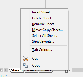
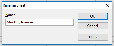
At the bottom of the window, right click on the sheet 1 tab and rename to ‘Monthly Planner’ and rename sheet 2 to ‘Important Dates’. Then right click and delete the third tab.
In the Important Dates tab, enter the word ‘Date’ in cell A1 and ‘Short Description’ in cell B1.
![]()
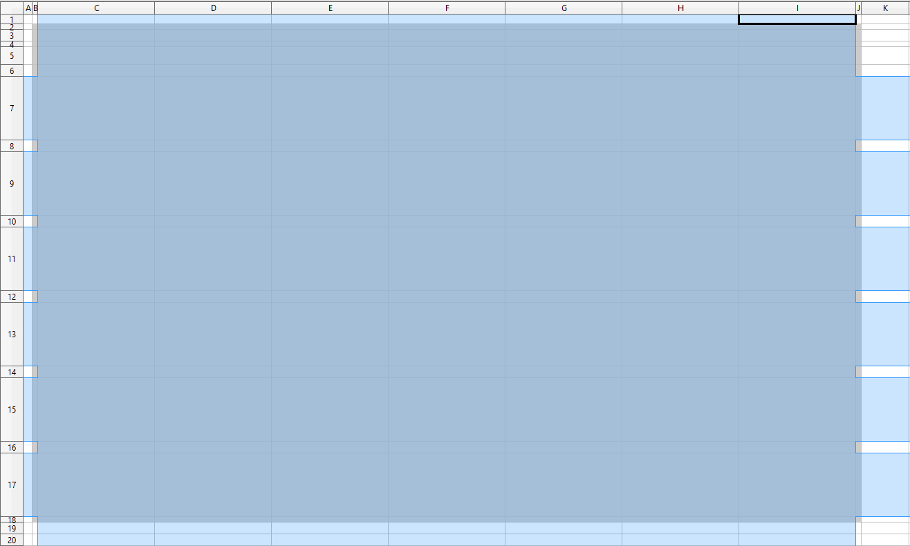
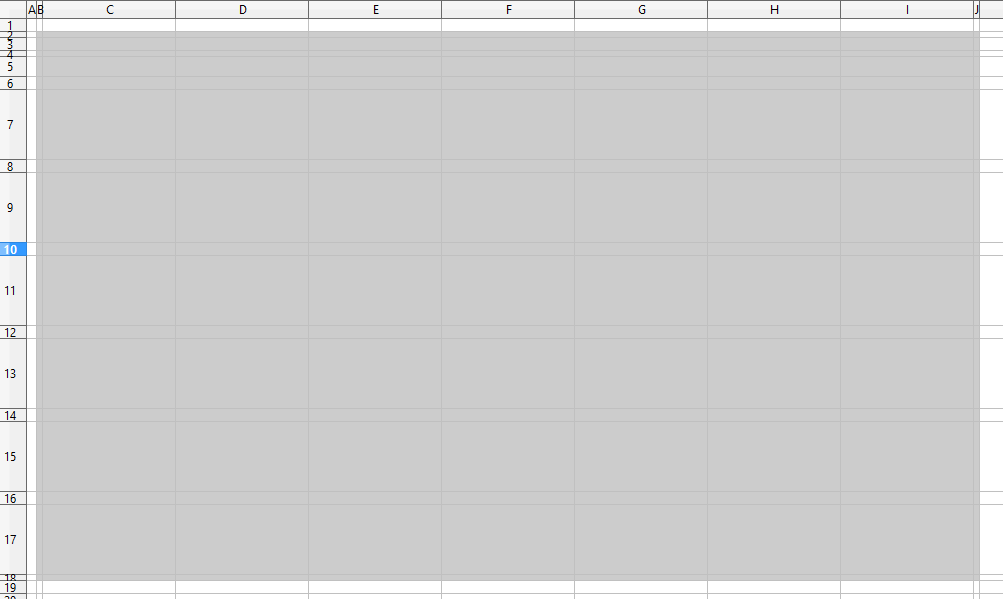
Now go to the Monthly Planner tab and adjust the cell width and heights. To resize multiple rows or columns at one time simple hold ctrl as you click on each letter or number, it will resemble something like the below image. This makes it easy to have each similar cell the same size.
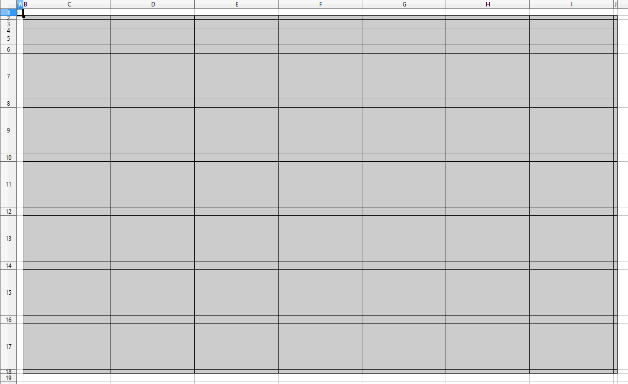
You should end up with something similar to below. I have added black borders to easily see the cell sizes and shapes.
Now select cell C3 and go to Data > Validity and change the Allow criteria from ‘All’ to ‘List’ and list the all 12 months of the year.
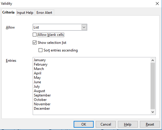
Click OK and you should have a nice drop down list. Now in cell D3 write the current year, you could also create another drop down list if you so prefer.

In cell C5 enter ‘Sunday’ and drag across to I5 (Saturday). To drag, hover your cursor over the bottom right hand corner of your selection bounds (the original cell) until your cursor turns into a plus sign.
![]()

Paste the following formulas in their corresponding cells. Where dragging is required, follow the same instructions as above.
|
Cell Destination |
Formula |
|
C6 |
=IF(WEEKDAY(DATEVALUE("1"&"-"&$C$3&"-"&$D$3))=1;1;IF(A6<>"";A6+1;"")) |
|
D6 |
=IF(WEEKDAY(DATEVALUE("1"&"-"&$C$3&"-"&$D$3))=2;1;IF(C6<>"";C6+1;"")) |
|
E6 |
=IF(WEEKDAY(DATEVALUE("1"&"-"&$C$3&"-"&$D$3))=3;1;IF(D6<>"";D6+1;"")) |
|
F6 |
=IF(WEEKDAY(DATEVALUE("1"&"-"&$C$3&"-"&$D$3))=4;1;IF(E6<>"";E6+1;"")) |
|
G6 |
=IF(WEEKDAY(DATEVALUE("1"&"-"&$C$3&"-"&$D$3))=5;1;IF(F6<>"";F6+1;"")) |
|
H6 |
=IF(WEEKDAY(DATEVALUE("1"&"-"&$C$3&"-"&$D$3))=6;1;IF(G6<>"";G6+1;"")) |
|
I6 |
=IF(WEEKDAY(DATEVALUE("1"&"-"&$C$3&"-"&$D$3))=7;1;IF(G6<>"";G6+1;"")) |
|
C7 drag to I7
|
=IF(C6<>"";IF(COUNTIF('Important Dates'.$A$2:$A$300;DATEVALUE(C6&"-"&$C$3&"-"&$D$3))>0;INDEX('Important Dates'.$B$2:$B$300;MATCH(DATEVALUE(C6&"-"&$C$3&"-"&$D$3);'Important Dates'.$A$2:$A$300;0));"");"")
|
|
C8 drag to I8 |
=I6+1 |
|
C9 drag to I9 |
=IF(C8<>"";IF(COUNTIF('Important Dates'.$A$2:$A$300;DATEVALUE(C8&"-"&$C$3&"-"&$D$3))>0;INDEX('Important Dates'.$B$2:$B$300;MATCH(DATEVALUE(C8&"-"&$C$3&"-"&$D$3);'Important Dates'.$A$2:$A$300;0));"");"")
|
|
C10 drag to I10 |
=I8+1 |
|
C11 drag to I11 |
=IF(C10<>"";IF(COUNTIF('Important Dates'.$A$2:$A$300;DATEVALUE(C10&"-"&$C$3&"-"&$D$3))>0;INDEX('Important Dates'.$B$2:$B$300;MATCH(DATEVALUE(C10&"-"&$C$3&"-"&$D$3);'Important Dates'.$A$2:$A$300;0));"");"")
|
|
C12 drag to I12 |
=I10+1 |
|
C13 drag to I13 |
=IF(C12<>"";IF(COUNTIF('Important Dates'.$A$2:$A$300;DATEVALUE(C12&"-"&$C$3&"-"&$D$3))>0;INDEX('Important Dates'.$B$2:$B$300;MATCH(DATEVALUE(C12&"-"&$C$3&"-"&$D$3);'Important Dates'.$A$2:$A$300;0));"");"")
|
|
C14 drag to I14 |
=IF(DAYSINMONTH(DATEVALUE("1"&"-"&$C$3&"-"&$D$3))>=C12+7;C12+7;"") |
|
C15 drag to I15 |
=IF(C14<>"";IF(COUNTIF('Important Dates'.$A$2:$A$300;DATEVALUE(C14&"-"&$C$3&"-"&$D$3))>0;INDEX('Important Dates'.$B$2:$B$300;MATCH(DATEVALUE(C14&"-"&$C$3&"-"&$D$3);'Important Dates'.$A$2:$A$300;0));"");"")
|
|
C16 drag to I16 |
=IF(C14<>"";IF(DAYSINMONTH(DATEVALUE("1"&"-"&$C$3&"-"&$D$3))>=C14+7;C14+7;"");"") |
|
C17 drag to I17 |
=IF(C16<>"";IF(COUNTIF('Important Dates'.$A$2:$A$300;DATEVALUE(C16&"-"&$C$3&"-"&$D$3))>0;INDEX('Important Dates'.$B$2:$B$300;MATCH(DATEVALUE(C16&"-"&$C$3&"-"&$D$3);'Important Dates'.$A$2:$A$300;0));"");"")
|
Select cell range C6:I17 and fill the background with a grey colour of your choice.
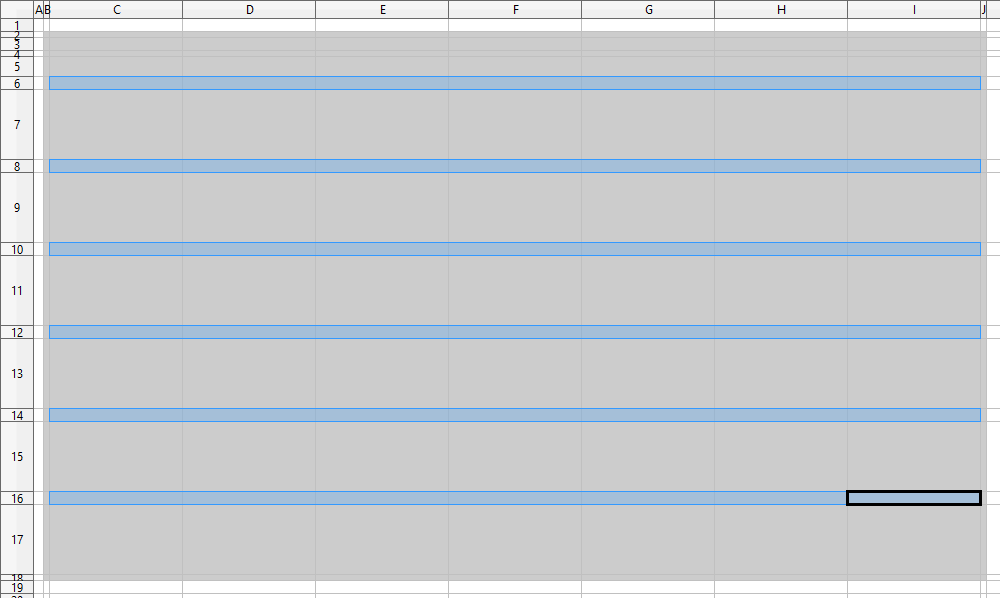
Then select the ranges C6:I6, C8:I8, C10:I10, C12:I12, C14:I14 and C16:I16 like below and go to format > conditional formatting.
Input the following details and click new style.
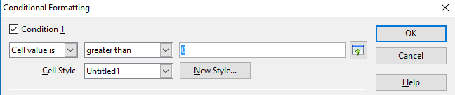
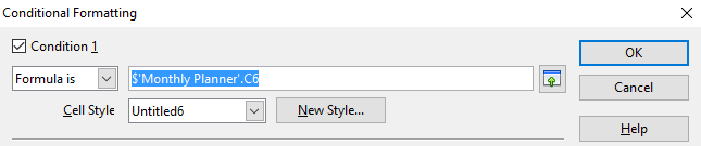
Customise the fill, font, border and alignment however you would like, here is an example.
Select the ranges C7:I7, C9:I9, C11:I11, C13:I13, C15:I15 and C17:I17 and ensure the top left cell of the selection is selected, like below.

Go to Format> Conditional formatting again. This time switch from ‘cell value’ to ‘formula is’. Then click on cell XX and remove the dollar signs from the formula. This is the cell addressing, we remove this so the formula applies to every cell we initially selected.
Then create a new style, I recommend using a white background here and a 10pt font size.
You should now have something that looks like this.

Now go to the Important Dates tab.
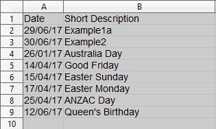
Populate this list with the important dates you wish to include in the planner. These could be assignment dates, public holidays, birthdays and/or sporting matches.
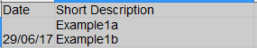
To populate more than one line on a single date simply double click on the description cell to edit then press ctrl + enter to split into two or more lines in the cell. It should end up looking like below.
After populating your dates, the planner is complete. Go to the cell properties and uncheck ‘Show cell grid lines’ to clean the look of the spreadsheets.
![]()

You can then print off the planner by selecting range B2:J18 in the Monthly Planner tab and go Format > Print Ranges > Define and then print to print that selection.